

Text Normalization with Machine Learning Method
CS5824 Machine Learning, Fall 2017, Final Project
Peng Peng
Shaohua Lei
Chun Wang

Many speeches and language applications, such as text-to-speech synthesis and automatic speech recognition, require text to be converted from written expressions into appropriate "spoken" forms [1, 2]. This process is known as text normalization. For example, the conversion from 1990 to "nineteen ninety" and $2.18 into "2 dollars, eighteen cents".
In real-world speech applications, the text normalization engine is developed, in large part, by hand [3]. Recently, deep learning method, such as Recurrent Neural Networks (RNN) and Long Short-Term Memory (LSTM) has been applied to this area [4, 5], although these models might produce prediction errors due to the inherent weakness of the method [6]. In addition, recent research shows that those errors can be mitigated using additional filters, such as finite-state transducer (FST) filter [4], and results in a level of accuracy not achievable by the RNN or LSTM alone. In this project, we applied LSTM for text normalization on a dataset recently released in Kaggle [7].
INTRODUCTION
Example records in this dataset are shown in Table 1.Each sentence in the dataset has a sentence_id, and each token within a sentence has a token_id. The “before” column contains the raw tokens, and the “after” column contains the tokens after text normalization. The column “class” shows the labeled class of the token.
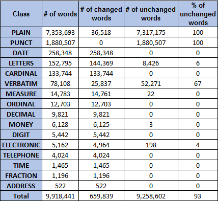
We have explored the dataset and summarized the basic statistics as shown in Table 2. There are 748,056 sentences in our training dataset, which consists of more than 9 million of words. In addition, there are 16 different labels for words in our dataset. Notably, the numbers of words with different labels are highly unbalanced. As shown in Table 2, most (more than 93%) of the words in our dataset belong to "PLAIN" or "PUNCT".
More importantly, we found that the majority of the tokens after text normalization remains unchanged. According to our statistic result, only about 7% of the tokens were changed during the text normalization. This percentage is class-dependent, for example, 100% of tokens in PUNCT and PLAIN classes are unchanged, while the tokens in DATE and CARDINAL are all changed after normalization.
Problem
Dataset
Table 1. Examples of input tokens in our dataset. The "before" and "after" are the tokens before and after normalization. The column "class" is the labeled class of the token.
Table 2. Statistic result on our dataset. There are 16 classes of words in our dataset and most of the tokens (more than 93%) are plain text word or punctuation. In addition, most of the tokens (~99%) are unchanged after normalization.


Figure 2. Visualization of our learned word embedding vectors using t-distributed stochastic neighbor embedding
Figure 1. Architecture of our LSTM model
-
Taylor, Paul. (2009). Text-to-Speech Synthesis. Cambridge University Press, Cambridge.
-
Ebden, Peter and Sproat, Richard. (2015). The Kestrel TTS text normalization system. Natural Language Engineering. 21(3).
-
Wu, K., Gorman, K., and Sproat, R. (2016). Minimally supervised written-to-spoken text normalization. arXiv 1609.06649.
-
Richard Sproat and Navdeep Jaitly. (2016). RNN Approaches to Text Normalization: A Challenge. Released on arXiv.org: https://arxiv.org/abs/1611.00068
-
Sundermeyer, Martin, Ralf Schlüter, and Hermann Ney. (2012). LSTM neural networks for language modeling. Thirteenth Annual Conference of the International Speech Communication Association.
-
Gers, Felix A., Jürgen Schmidhuber, and Fred Cummins. (1999). Learning to forget: Continual prediction with LSTM. 850-855.
-
https://www.kaggle.com/c/text-normalization-challenge-english-language
REFERENCE

In this project, we performed text normalization using machine learning method. Our machine learning model was a recurrent neural network consisted of sequential layers as shown in Figure 1. The first layer of our model was an LSTM layer which consisted of 128 LSTM units. The LSTM layer was followed by fully connected dense layers with the 32 ReLU activation function units. Then a soft-max layer was employed to generate the class label for the input token.
Before entering our RNN, the input tokens were transferred to vectors using the word2vector embedding method. The embedding model we used is based on the skip-gram model with the optimization of noise-contrastive estimation loss. After embedding, each token in our dataset was represented by a vector with 32 dimensions. After training our embedding model, we visualized the learned word embedding result as shown in Figure 2. We found that the resulting vectors for similar words end up clustering nearby each other. For example, the numbers for years were grouping together and were separated with the other numbers. Therefore we believed that this feature extraction using word embedding would help our text normalization process.
Both our embedding model and sequential multilayer RNN model were created using Keras API for Python using the TensorFlow backend.
FEATURE & MODEL
EVALUATION
Firstly, we designed a simple and straightforward statistical model as a baseline to evaluate our LSTM model. This model is based on creating a dictionary with all the tokens in our training set as keys, while the values are the most frequently used normalized tokens for the corresponding key tokens. When training the baseline model, we simply recorded and counted all possible outputs for each token. During the testing, if the token was in the trained dictionary, we took the corresponding most frequently used the normalized token as its output; otherwise, the original token would be used as the output.
Surprisingly, the accuracy of this really simple baseline model could reach a score more than 94%. This is because our dataset are highly unbalanced. According to Table 2, most of the tokens are with the label of "PLAIN" or "PUNCT", and the tokens with both labels are normalized to themselves. According to Table 2, 93% of the original tokens remain unchanged after normalization, which means that even if we simply keep every tokens unchanged during normalization, we could still get the accuracy of over 93%. This results indicated that accuracy is not a good metrics for our task of text normalization. Therefore, we used F1 score instead to measure the performance of both models. To clarify, we took unchanged tokens after normalization as negative samples and the changed tokens as positive samples. Finally, we tested our baseline model and LSTM model using 10-fold cross validation, and got the average F1 score for each module.
According to our calculated F1 score as shown in Table 3, the baseline model resulted in few false positive samples but a large number of false negative samples. Therefore the F1 score is only around 25%. This is reasonable because for according to the statistical result, a token is more likely to remains unchanged in the training data. In addition, most of the tokens that need to change are relatively rare, such as the numbers, telephone numbers, addresses. These tokens are less likely to duplicate in both training and testing dataset, which will be predicted to unchanged tokens by our baseline model. In other words, the baseline model tended to keep tokens unchanged, which resulted in higher false negative.
On the other hand, for the LSTM model, our model got a much higher F1 score around 60%. According to Table 3, our LSTM model greatly increased the true positive samples and also reduced false negative samples. Although the LSTM reduced the number of true negative samples, the resulting accuracy and F1 scores of our LSTM are both better than our baseline model.

Table 3. Results of baseline and LSTM models. TP: true positive samples; FP: false positive samples; FN: false negative samples; TN: true negative samples.